Bayesian Modeling

class: center, middle, inverse, title-slide

# Bayesian Modeling
## with R2jags
### Zhi Yang
### 2019-04-08

---

# A mini GO~~T~~B  family tree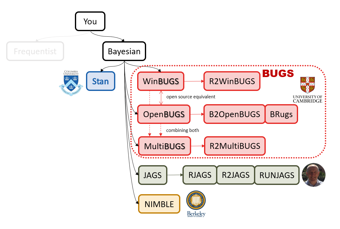

![](imgs/history.png)
---
# What'll be in this talk

#### Some history about tools for Bayesian modeling
#### Bayes' theorem, jargons and Shiny demo (prior, posterior ...)
#### A walkthrough of using `R2jags` (meetup pizza example)
#### More examples (linear regression)

---
class: center, middle
# .red[Why Bayesian?]

### You learn from the data

### You know the uncertainty of the estimated parameters

.left[.footnote[[My Journey From Frequentist to Bayesian Statistics](http://www.fharrell.com/post/journey/)]]
---

class: center, middle

#.red[JAGS]

###stands for

#.red[Just Another Gibbs Sampler]

### developed by Martyn Plummer 
<img src="imgs/mp.jpg" width="20%">

---
class: center, middle

#.red[Why JAGS?]

###why not WinBUGS 🐞 or Stan?

---
#JAGS vs. WinBUGS

### WinBUGS is historically very important with slow development

### JAGS has very similar syntax to WinBUGS and it allows cross-platform

### Great interface to **.blue[R]**! .small[(rjags, R2jags,runjags)]

.footnote[ [When there is WinBUGS already, why is JAGS necessary?](https://www.quora.com/When-there-is-WinBUGS-already-why-is-JAGS-necessary) ]

---
.pull-left[
# .red[JAGS]
* longer history with tons of resources 📕📝🎓
* easy to learn and run it
* need to recompile model
* fewer developers
* less viz tools
* various MCMC sampling methods
]
.pull-right[
# .blue[Stan]
* A newer tool with great team/active community
* steeper learning curve 
* no need to recompile
* Syntax check in **.blue[R]** 😱
* ShinyStan (applicable to JAGS)
* require fewer iterations to converge
]

.center[### Which one's faster? Inconclusive]
### .red[My situation] Stan doesn't support discrete sampling

.footnote[
[Stan vs. WinBugs: A search for informed opinions](https://www.reddit.com/r/statistics/comments/5on87q/stan_vs_winbugs_a_search_for_informed_opinions/)
]

---
#.red[Why me?]
### I wrote a part of my dissertation with **JAGS**

### I've repeatedly read through **JAGS**, WinBUGS manual and numerous journals

### I've four years' experiences with searching **JAGS** examples in Google and GitHub

---
# Installation

### Install **R**

### Install **RStudio**

### Install the **JAGS** from https://sourceforge.net/projects/mcmc-jags/

### Install the **R2jags** package from [CRAN](https://cran.r-project.org/web/packages/R2jags/index.html):

```r
install.packages("R2jags")
library(R2jags)
```

---
#30 seconds on Bayes' theorem
.pull-left[
![](https://cdn-images-1.medium.com/max/1600/1*oKi6F9CNeCyhLajj_RRSoA.jpeg)
]

.pull-right[
Changing our beliefs based on evidences
`$$Posterior = \frac{Likelihood \times Prior}{Evidence}$$`
]

### Prior: strong vs. weak ? <br>
### Data: insufficient vs. sufficient ?

.footnote[[Nat Napoletano:Bayes' Theorem for Everyone](https://www.youtube.com/watch?v=XR1zovKxilw)]

---
# Shiny Demo

The focus of the analysis presented here is on accurately estimating the mean of IQ using simulated data.

[FBI: First Bayesian Inference](https://www.rensvandeschoot.com/fbi-the-app/)

.footnote[https://www.ncbi.nlm.nih.gov/pmc/articles/PMC4158865/]

---
# Strong prior vs. weak prior

![](https://cdn-images-1.medium.com/max/800/1*YN48zFbH6sEpOe-cbBjfbg.gif)
![](https://cdn-images-1.medium.com/max/800/1*RV087VG2ntly7mIEEML2oQ.gif)

.footnote[https://towardsdatascience.com/visualizing-beta-distribution-7391c18031f1]

---
# Let's get started!
We hold meetings every month and post it on meetup.com, which tells us how many people've signed up, `$n$`. But not everyone show up (i.e., traffic). So, we'd like to know what percentage of people, `$\theta$`,  will show up to order enough pizzas.

.center[
`$Y_i|\theta \sim Binom(n_i, \theta)$`

`$\theta \sim Beta(a, b)$` 
]

Weak prior: 
.center[
`$Beta(1, 1) \leftrightarrow Unif(0, 1)$`
]

```r
Y <- c(77, 62, 30)
N <- c(39, 29, 16)
```

---
# Write the model

But as you know, someone (@lukanegoita) said

---
# Write the model
.center[
`$Y_i|\theta \sim Binom(n_i, \theta)$`

`$\theta \sim Beta(a, b)$`

]

.pull-left[
In .blue[R]
```r
model{
for(i in 1:3){
  Y[i] <- rbinom(1, N[i], theta) 
}
  theta <- rbeta(1, 1, 1)
}
```
]

.pull-right[
In .red[JAGS]
```r
model{
for(i in 1:3){
  Y[i] ~ dbinom(theta, N[i])
}
  theta ~ dbeta(1, 1)
}
```
]

- A variable should appear **only once** on the left hand side
- A variable may appear multiple times on the right hand side
- variables that only appear on the right must be supplied as **data**

---
# Tips on syntax 
#### No need for variable declaration
#### No need for semi-colons at end of statements
#### use d`dist` instead of r`dist` for random sampling
#### dnorm(mean, **precision**) .red[not] dnorm(mean, **sd**)
#### It allows matrix and array
#### It is .red[illegal] to offer definitions of the variable twice

---
# Write the model

```r
suppressMessages(library(R2jags))
model_string <-"
model{
# Likelihood
for(i in 1:3){
  Y[i] ~ dbinom(theta, N[i])
}

# Prior
  theta ~ dbeta(1, 1)
}
"

# Data
N <- c(77, 62, 30)
Y <- c(39, 29, 16)

# specify parameters to be monitered
params <- c("theta")
```

---
# rjags vs. runjags vs. R2jags
#### `R2jags` and `runjags` are just wrappers of rjags
#### `runjags` makes it easy to run chains in parallel on multiple processes
#### `R2jags` allows running until converged and paralleling MCMC chains
#### Otherwise, they all have very similar syntax and pre-processing steps

---
# Choosing `R2jags`

```r
output <- jags(model.file = textConnection(model_string), 
               data = list(Y = Y, N = N),
               parameters.to.save = params,
               n.chains = 2, n.iter = 2000)
```

```
## Compiling model graph
##    Resolving undeclared variables
##    Allocating nodes
## Graph information:
##    Observed stochastic nodes: 3
##    Unobserved stochastic nodes: 1
##    Total graph size: 9
## 
## Initializing model
## 
## 
  |                                                        
  |                                                  |   0%
  |                                                        
  |**                                                |   4%
  |                                                        
  |****                                              |   8%
  |                                                        
  |******                                            |  12%
  |                                                        
  |********                                          |  16%
  |                                                        
  |**********                                        |  20%
  |                                                        
  |************                                      |  24%
  |                                                        
  |**************                                    |  28%
  |                                                        
  |****************                                  |  32%
  |                                                        
  |******************                                |  36%
  |                                                        
  |********************                              |  40%
  |                                                        
  |**********************                            |  44%
  |                                                        
  |************************                          |  48%
  |                                                        
  |**************************                        |  52%
  |                                                        
  |****************************                      |  56%
  |                                                        
  |******************************                    |  60%
  |                                                        
  |********************************                  |  64%
  |                                                        
  |**********************************                |  68%
  |                                                        
  |************************************              |  72%
  |                                                        
  |**************************************            |  76%
  |                                                        
  |****************************************          |  80%
  |                                                        
  |******************************************        |  84%
  |                                                        
  |********************************************      |  88%
  |                                                        
  |**********************************************    |  92%
  |                                                        
  |************************************************  |  96%
  |                                                        
  |**************************************************| 100%
```

---
# Visualizing output

```r
plot(as.mcmc(output))
```

![](index_files/figure-html/unnamed-chunk-7-1.png)

---
# Visualizing output

```r
library(mcmcplots)
mcmcplot(as.mcmc(output),c("theta"))
denplot(as.mcmc(output),c("theta"))
```

![](imgs/mcmcplots.png)

---
# Model diagnostic 
So it might take a longer time for run

---
## Model diagnostic and convergence

```r
output$BUGSoutput$summary
```

```
##                mean         sd       2.5%        25%       50%        75%
## deviance 14.6685495 1.42564249 13.6497484 13.7569065 14.104791 15.0374241
## theta     0.4962242 0.03867905  0.4226714  0.4693877  0.496706  0.5209497
##               97.5%     Rhat n.eff
## deviance 18.7817874 1.002871   630
## theta     0.5723382 1.000970  2000
```

If it fails to converge, we can do the following,

```r
update(output, n.iter = 1000)
autojags(output, n.iter = 1000, Rhat = 1.05, n.update = 2)
```

---
# weak prior vs. strong prior

```r
output$BUGSoutput$summary
```

```r
output2$BUGSoutput$summary
```

```
##                mean        sd       2.5%        25%        50%        75%
## deviance 15.2204981 1.7165810 13.6500147 13.9259913 14.6814049 15.9249686
## theta     0.5346611 0.0298314  0.4752045  0.5146234  0.5355181  0.5547805
##              97.5%     Rhat n.eff
## deviance 19.846200 1.000531  2000
## theta     0.591993 1.000510  2000
```

---
# weak prior vs. strong prior
.pull-left[

```r
denplot(as.mcmc(output), 
         parms = "theta", 
         xlim = c(0.3, 0.7))
```

![](index_files/figure-html/unnamed-chunk-12-1.png)
]
.pull-right[

```r
denplot(as.mcmc(output2), 
        parms = "theta", 
        xlim = c(0.3, 0.7))
```

![](index_files/figure-html/unnamed-chunk-13-1.png)
]

---
# linear regression 
.pull-left[
In .red[JAGS]
```r
model<-"model{
# Likelihood
for(i in 1:N){
  y[i] ~ dnorm(mu[i], tau)
  mu[i] <- beta0 + beta1*x[i]
}

# Prior
  # intercept
  beta0 ~ dnorm(0, 0.0001)
  # slope
  beta1 ~ dnorm(0, 0.0001)
  # error term
  tau ~ dgamma(0.01, 0.01)
  sigma <- 1/sqrt(tau)
}"
```

In statistics 101

`$Y_i = b_0 + b_1X_i + \sigma$`
`$Y \sim N(b_0 + b_1X, \sigma^2)$`

<br>
]

.pull-right[
In .blue[R]

```r
lm(y~x)
```
]

```
## Compiling model graph
##    Resolving undeclared variables
##    Allocating nodes
## Graph information:
##    Observed stochastic nodes: 15
##    Unobserved stochastic nodes: 3
##    Total graph size: 74
## 
## Initializing model
```

---
# Interpretation

.pull-left[
In .red[JAGS]

```r
lm_output$BUGSoutput$summary[1:2, c(3,7)]
```

```
##             2.5%     97.5%
## beta0  -8.853992 52.131691
## beta1 -16.496277  3.192873
```

95% credible interval
]

.pull-right[
In .blue[R]

```r
confint(lm(y~x))
```

```
##                 2.5 %    97.5 %
## (Intercept)  -9.32782 51.322335
## x           -16.19329  3.486528
```

95% confidence interval
]

---
# Resources 📕+💻
.pull-left[
#### If you've got 2hrs: 
 - useR! International R User 2017 Conference JAGS [workshop](https://channel9.msdn.com/Events/useR-international-R-User-conferences/useR-International-R-User-2017-Conference/Introduction-to-Bayesian-inference-with-JAGS) by Martyn Plummer <-- 👨 of **JAGS**
]

.pull-right[
#### If you've got 5 mins:
[RJAGS: how to get started](https://www.rensvandeschoot.com/tutorials/rjags-how-to-get-started) by Rens van de Schoot, retweeted by Martyn Plummer
]

#### <center>  If you're a book lover:
<center><img src="imgs/book2.png" width=25%> <img src="imgs/book.jpg" width=26%>

---
# What about puppies?

"perky ears" + "floppy ears"  ?= "half-up ears"

---
# More ...

- [CRAN Task View: Bayesian Inference](https://cran.r-project.org/web/views/Bayesian.html)
- ["Selling" Stan](https://discourse.mc-stan.org/t/selling-stan/3693/9)

### Meet greta 
For those still can't decide which any external tool?

- [greta](https://greta-stats.org/index.html) allows you to write models without learning another language like BUGS or Stan
- It uses Google TensorFlow (fast!)
![](https://greta-stats.org/reference/figures/main_icon.png)

---
# greta example
![](imgs/greta.png)